![]()
Open-Source Seismic Hazard Analysis (OpenSHA)
Glossary
The following is a list of terms commonly used in OpenSHA and in seismic hazard analysis in general.
Table Of Contents
- Attenuation Relationship
- Distance
- Earthquake Rupture
- Earthquake Rupture Forecast (ERF)
- Epsilon
- Fault
- Frankel Fault Surface
- GCIM
- Gridded Surface
- Ground Motion Prediction Equation (GMPE)
- Hanging Wall & Foot Wall
- Hazard Data
- Intensity Measure (IM)
- Intensity Measure Relationship (IMR)
- Intensity Measure Type (IMT)
- Magnitude
- Magnitude Frequency Distribution (MFD)
- Magnitude Scaling Relationship
- NGA Models
- Probabilistic Earthquake Source
- Rupture Surface
- Shaking Component
- Shear Wave Velocity (Vs)
- Sigma Truncation
- Simple Fault
- Site
- Standard Deviation
- Stirling Fault Surface
- Strike, Dip, & Rake (Focal Mechanism)
- Tectonic Regime
- Wills Site Classification
Attenuation Relationship
An Attenuation Relationship is a type of Intensity Measure Relationship (IMR) that assumes the Intensity Measure Level (IML) (or logarithm thereof) is both a scalar and exhibits a Gaussian distribution. The mean and standard deviation of the Gaussian distribution (and exceedance probabilities derived therefrom) are computed from various parameters, the types of which are discussed below. Of course by virtue of being an Intensity Measure Relationship (IMR), the mean and standard deviation can also be computed from a given Site and Earthquake Rupture. Attenuation relationships are sometimes referred to as Ground Motion Prediction Equations (GMPEs). There are no limits on what types of parameters an attenuation-relationship author can choose to make their model depend upon. However, the following gives the various categories these parameters must fall under, as well as a few common examples for each:
Earthquake Rupture Parameters
These parameters are obtained or computed from a given Earthquake Rupture and include:
- Magnitude(MW)
- Average Rake
- Average Dip
- Rupture Top Depth
Site Parameters
Site-specific parameters that may include:
Propagation-Effect
These parameters are computed from a given Site and Earthquake Rupture and may include:
- Distance
- Hanging-Wall Data
- Directivity Data
Other
Parameters common to many attenuation relationships that don’t fall into the categories above:
- Component (e.g., Avg. Horizontal, GMRotI50, Vertical, Random Horizontal, Greater of Two Horizontal)
- Standard Deviation Type (e.g., Total, Inter-Event, Intra-Event, Zero)
- Sigma Truncation Type (e.g., None, One-Sided, Two-Sided)
- Sigma Truncation Level
Parameter values are numeric unless otherwise indicated with options.
Distance
In OpenSHA, Distance refers to the distance between an Earthquake Rupture and a Site. However, many Attenuation Relationships use different criteria to define distance. These are the currently supported definitions:
DistanceRup
The shortest distance from a site to a rupture surface.
DistanceSeis
The shortest distance from a site to a point on a rupture surface that is deeper than some minimum seismogenic depth.
DistanceJB
The Joyner-Boore distance defined as the shortest distance from a site to the surface projection of the rupture surface.
DistanceX
The shortest horizontal distance from a Site to a line defined by extending the fault trace (or the top edge of the rupture) to infinity in both directions. Values on the hanging-wall are positive and those on the foot-wall are negative.
(distRup - distJB) / distRup
The difference between DistanceRup and DistanceJB (normalized by DistanceRup).
(distRup - distX) / distRup
The difference between DistanceRup and DistanceX (normalized by DistanceRup).
See entry on Earthquake Rupture for definition of terms: rupture surface, seismogenic depth, fault trace, hanging-wall, foot-wall
Earthquake Rupture
 (click to enlarge)
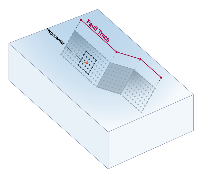
In OpenSHA, an Earthquake Rupture refers to an event that generates seismic energy as a result of slip on a fault. For large and relatively well-studied events, a rupture may be represented as a portion of a fault that slips during the event. For smaller and less well-studied events, a rupture may be represented simply as a point source. An Earthquake Rupture is defined by a:
- Magnitude(MW)
- Average Rake
- Rupture Surface
- Tectonic Regime
- Hypocenter (optional)
Hypocenter
A location on a Rupture Surface that marks where earthquake slip nucleates.
Probabilistic Earthquake Rupture
An Earthquake Rupture with an associated probability of occurrence. See also Probabilisitic Earthquake Source.
Earthquake Rupture Forecast (ERF)
 (click to enlarge)
An Earthquake Rupture Forecast (ERF) is one of the two main modeling components in OpenSHA, the other being an Intensity Measure Relationship (IMR). An ERF gives a forecast of all possible Earthquake Ruptures) as their probability of occurrence over a specified Time Span. In OpensSHA, an ERF is given as a list of Probabilistic Earthquake Sourcess) and includes information on its region of applicability.
Epsilon
Given an earthquake with a specified magnitude and distance from a site of interest, Epsilon is a measure of how ground motion deviates from the expected mean. In most cases, one is interested in a ground motion that has a probability of being exceeded over some time period. This is often quite different than the most likely (or mean) ground motion that would be experienced if the event were to occur at any time and epsilon characterizes this variability. Please see the USGS Deaggregation site for more detailed information and references
Fault
In the context of OpenSHA, a fault is a relatively planar surface or discontinuity in the earth that can accomodate slip that manifests as earthquakes (see Wikipedia for more info on faults). OpenSHA describes fault geometries in several ways:
Simple Fault Type
The most common type of fault representation in OpenSHA is that of a Simple Fault. A Simple Fault encapsulates the basic information required to define a fault geometry and is one possible basis for Gridded Surfaces such as the Frankel and Stirling Fault Surfaces.
Other Fault Types
OpenSHA can accomodate these additional fault types:
- Subduction Zones (see the USGS SLAB project)
- Listric Faults
These other fault types may also be gridded.
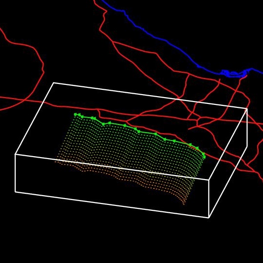
Frankel Fault Surface
 (click to enlarge)
A Frankel Fault Surface is one representation of a Gridded Surface that was created by Arthur Frankel for use in the 1996 and 2002 USGS National Seismic Hazard Maps. See also Earthquake Rupture. In OpenSHA, the trace and average dip of a Simple Fault are used to create rectangular surfaces where the dip direction of each rectangle is perpendicular to the strike of its local segment. The resulting surface is then gridded (discretized) according to whatever interval is specified. Compare to a Stirling Fault Surface.
GCIM
The Generalized Conditional Intensity Measure (GCIM) provides a multi-variate distribution of ground motion intensity measures conditional on a specific value of a single intensity measure. A ground motion selection algorithm can automatically select ground motions based on the GCIM distributions. GCIM distributions can be calculated in the OpenSHA HazardCurve application. See Ground motion selection by Brendon A. Bradley to learn more.
Gridded Surface
 (click to enlarge)
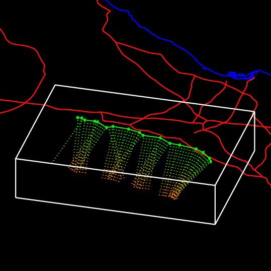
To facilitate modeling larger earthquakes of various sizes, OpenSHA treats fault and rupture surfaces as gridded surfaces. Gridding makes it easier to both represent arbitrary degrees of surface complexity, and to reference a subset of a larger surface (e.g., for when an Earthquake Rupture occurs on only part of a fault). Depending on the type of Fault being gridded, OpenSHA can accomodate evenly discretized grids (e.g. the fault surface definitions of Frankel and Stirling) or approximately uniformely spaced grids (e.g., for subduction zones).
Ground Motion Prediction Equation (GMPE)
This is synonymous with Attenuation Relationship (OpenSHA uses the latter).
Hanging Wall & Foot Wall
For a dipping fault, the Hanging Wall is the block positioned over the fault, the Foot Wall is the block positioned under it. See the cross-sections below and the Wikipedia entry on faults for more information.

More information related to faults can be found in the Rupture Surface and Strike Dip, & Rake glossary entries.
Hazard Data
Output from seismic hazard calculations generally takes two forms:
Hazard Curve
A plot of the probability of exceedance versus an Intensity Measure Level (IML) for a specified Intensity Measure Type (IMT).
Hazard Map
A map view of the probability that an IMT will exceed a specified IML, or the IML that has a specified probability of being exceeded (the former is actually the correct definition, but the latter is commonly used as well).
Intensity Measure (IM)
An Intensity Measure is an attribute of earthquake shaking that is useful for predicting damage or loss. It is defined by an:
Intensity Measure Type (IMT)
An IMT specifies the particular type of Intensity Measure. IMTs currently implemented in OpenSHA include:
- Peak Ground Acceleration (PGA)
- Peak Ground Velocity (PGV)
- Peak Ground Displacement (PGD)
- Spectral Acceleration (SA)
- Modified Mercalli Intensity (MMI)
OpenSHA was designed so that virtually any other IMT may be defined and implemented. For example, a new IMT might be composed of a vector of traditional IMTs.
Intensity Measure Level (IML)
An IML specifies the level, or value, of the IMT that one is concerned about exceeding. For example, one might want to know that probability that Peak Ground Velocity (the IMT) will exceed a level of 100 cm/sec (the IML).
Intensity Measure Relationship (IMR)
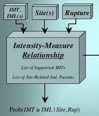
An Intensity Measure Relationship (IMR) is one of the two main modeling components in OpenSHA, the other being an Earthquake Rupture Forecast (ERF). An IMR gives the probability of exceeding some Intensity Measure Level (IML) of a specified Intensity Measure Type (IMT) given a Site of interest and an Earthquake Rupture.
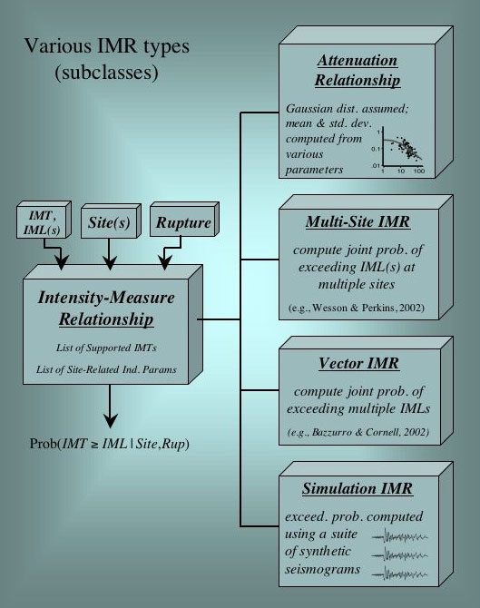 (click to enlarge)
Note that no presumptions are made with respect to how probabilities are computed, leaving the possibility of using full waveform modeling from first principles of physics. At present most IMRs implemented in OpenSHA constitute empirical Attenuation Relationships, although waveform modeling is being implemented in collaboration with the SCEC CyberShake project. See the figure at right for information on other potential types of IMRs.
Intensity Measure Type (IMT)
The Intensity Measure Types supported in OpenSHA include:
Peak Ground Acceleration (PGA)
The peak ground acceleration during an earthquake measured in units of ‘g’ (gravity).
Peak Ground Velocity (PGV)
The peak ground velocity during an earthquake measured in units of ‘cm/sec’ (cgs)
Peak Ground Displacement (PGD)
The peak ground displacement during an earthquake measured in units of ‘cm’ (cgs).
Spectral Acceleration (SA)
The maximum acceleration of a damped, single-degree-of-freedom harmonic oscillator, measured in units of ‘g’ (gravity). Spectral acceleration is an approximate measure of what is experienced by a building during an earthquake and is further specified by:
- Spectral Period: the natural period (seconds) of the oscillator
- Spectral Damping: the degree of damping for the oscillator (usually 5%)
More information on SA is available at the USGS.
Modified Mercalli Intensity (MMI)
A Roman numeral describing the severity of an earthquake in terms of its effects on the earth’s surface and on humans and their structures (see also Wikipedia).
See also Intensity Measure
Magnitude
In OpenSHA “Magnitude” is synonymous with “Moment Magnitude” (in keeping with the USGS Earthquake Magnitude Policy). Moment Magnitude = (log(Seismic Moment) - 9.05)/1.5 where Seismic Moment is given in SI units (Newton-meters).
Magnitude Frequency Distribution (MFD)
A Magnitude Frequency Distribution is a function that describes the rate (per year) of earthquakes across all magnitudes. An MFD can have an analytical form or, as in the case of OpenSHA implementations, be described by rates of earthquakes over descrete intervals. In addition to an arbitrary distribution, the following types of distributions are currently supported in OpenSHA:
- Single-Mag Distribution
- Gutenberg-Richter Distribution
- Tapered Gutenberg-Richter Distribution
- Gaussian Distribution
- Youngs and Coppersmith Distribution (AKA the”Characteristic” Distribution)
- Summed Magnitude Frequency Distribution (the sum of other distributions)
One can learn more about these using the Magnitude-Frequency Distribution Plotter.
Magnitude Scaling Relationship
A magnitude-scaling relationship gives mean Magnitude as a function of rupture area or length (or visa versa), where length and area are given in units of km and km-sq, respectively. Currenly Implemented Magnitude-Area Relationships:
- Wells and Coppersmith (1994, Bull. Seism. Soc. Am.):
- Mag = 4.07+0.98*log(Area) (all rupture types)
- Mag = 3.98+1.02*log(Area) (strike slip rupture)
- Mag = 4.33+0.90*log(Area) (reverse or thrust rupture)
- Mag = 3.93+1.02*log(Area) (normal rupture)
- Area = 10\^(-3.49+0.91*Mag) (all rupture types)
- Area = 10\^(-3.42 + 0.90*Mag) (strike slip rupture)
- Area = 10\^(-3.99 + 0.98*Mag) (reverse or thrust rupture)
- Area = 10\^(-2.87 + 0.82*Mag) (normal rupture)
- Uncertainty on Mag is 0.24, 0.23, 0.25, and 0.25 for all, strike slip, reverse, and normal ruptures, respectively.
- Uncertainty on log(Area) is 0.24, 0.22, 0.26, and 0.22 for all, strike slip, reverse, and normal ruptures, respectively.
- Hank & Bakun (2002 & 2008, Bull. Seism. Soc. Am.)
- Mag = 3.98+log(Area) (if Area <= 537)
- Mag = 3.07+(4/3)*log(Area) (if Area > 537)
- These equations are inverted to get Area from Mag
- No uncertainty estimates given
- Ellsworth (2003, published in Chapter 4 and Appendix D of the 2002 Working Group on California Earthquake Probabilities)
- Mag = 4.1+log(Area) (Equation 4.5a, AKA “Ellsworth A”)
- Mag = 4.2+log(Area) (Equation 4.5b, AKA “Ellsworth B”)
- Mag = 4.3+log(Area) (Equation 4.5c, AKA “Ellsworth C”)
- These equations are inverted to get Area from Mag
- Uncertainty on Mag is 0.1
Currenly Implemented Magnitude-Length Relationships:
- Wells and Coppersmith (1994, Bull. Seism. Soc. Am.):
- Mag = 5.08+1.16*log(Length) (all rupture types)
- Mag = 5.16+1.12*log(Length) (strike slip rupture)
- Mag = 5.00+1.22*log(Length) (reverse or thrust rupture)
- Mag = 4.86+1.32*log(Length) (normal rupture)
- Length = 10\^(-3.22+0.69*Mag) (all rupture types)
- Length = 10\^(-3.55+0.74*Mag) (strike slip rupture)
- Length = 10\^(-2.86+0.63*Mag) (reverse or thrust rupture)
- Length = 10\^(-2.01+0.50*Mag) (normal rupture)
- Uncertainty on Mag is 0.28, 0.28, 0.28, and 0.34 for all, strike slip, reverse, and normal ruptures, respectively.
- Uncertainty on log(Length) is 0.22, 0.23, 0.20, and 0.21 for all, strike slip, reverse, and normal ruptures, respectively.
NGA Models
These are the Attenuation Relationships developed as part of the PEER “Next Generation Attenuation” (NGA) project.
Available Models
Implementation Verification
To provide independent verification of OpenSHA’s implementations of the NGA models, Kenneth Campbell (EQECAT Inc.) computed a suite of test files. These files provide mean and standard-deviation values for a sufficiently wide range of parameter settings to suggest that OpenSHA implementations are correct, or at least consistent with independent computations. The test files and README are available here (2.8 MB .zip file). The tests include ~170,000 test calculations, the results of which all of which match to within 0.05%. Each file has a single-line header to label the columns. The first nine columns represent values of the following parameters:
- Mw - Magnitude
- Rrup - DistanceRup (km)
- Rjb - DistanceJB (km)
- Rx - DistanceX (km)
- Dip - Average Dip of the rupture plane (degrees)
- W - Down Dip Width of rupture plane (km)
- Ztor - Rupture Top Depth (km)
- Vs30 - Vs30 (m/sec)
- Zsed - Depth 1.0 km/sec or Depth 2.5 km/sec depending on the model (km)
(note that not all the above are used by each NGA model) The columns that follow represent the mean or natural-log standard deviation for various spectral periods, SA (g), plus PGA (g) and PGV (cm/s). There are 30 separate files for testing: different NGA models, different focal mechanisms, mean versus standard deviation (sigma), whether sites are on the hanging wall, whether the event is an aftershock, and whether Vs30 is measured or inferred/estimated.
Probabilistic Earthquake Source
A Probabilistic Earthquake Source is a list of mutually exclusive Probabilistic Earthquake Ruptures. As an example, a Probabilistic Earthquake Source could be defined for a particular fault as a list of all possible Earthquake Ruptures corresponding to a range of Magnitudes that could occur on the fault or Rupture Surface. A Probabilistic Earthquake Source can also encapsulates the following information:
- Number of Probabilistic Earthquake Ruptures in the list
- Total Probability (sum of those in the list)
- Total Probability above a specified Magnitude
- Whether or not the source is Poisson (if yes, the probability for each Probabilistic Earthquake Rupture is interpreted as the probability of one or more events, otherwise it’s interpreted as the probability of the next event)
A Probabilistic Earthquake Source is also always defined in the context of an Earthquake Rupture Forecast (ERF), so the event probabilities are with respect to the Time Span associated with the ERF.
Rupture Surface
 (click to enlarge)
In OpenSHA, a Rupture Surface is the surface that slips during an earthquake (see Earthquake Rupture). It may be represented in a variety of ways:
- Point Surface – Used to represent point-source earthquakes.
- Gridded Surface – Used to represent entire faults (e.g. the uniformely gridded Frankel Fault Surface, Stirling Fault Surface, and Listric Surface. We also have an Approximately Gridded Surface that is used for subduction zones).
- Subset Surface – Used to represent subsets of entire Gridded Surfaces (see figure to right) when modelling earthquakes of different sizes on an individual fault.
A Fault Surface is further defined by a:
Rupture Top Depth
The depth (in km) to the shallowest point on an earthquake Rupture Surface.
Down Dip Width
The average width of an Rupture Surface measured in the down-dip direction.
Shaking Component
The Component of shaking of interest for an Intensity Measure (IM). Current options in OpenSHA include:
Average Horizontal
Usually defined as the geometric average of the maximum of the two horizontal components (which may not occur at the same time).
Average Horizontal (GMRotI50)
Because Average Horizontal, above, is dependent on seismometer orientation, this was defined by Boore et al. (2006, Bull. Seism. Soc. Am. 96, 1502-1511).
Random Horizontal
A randomly chosen horizontal component.
Vertical
The vertical component.
Greater of Two Horizontal
The largest value obtained from two perpendicular, horizontal components.
Shear Wave Velocity (Vs)
In seismic hazard analysis, the Shear Wave Velocity at a Site is of interest because it gives an indication of whether the expected shaking in response to an Earthquake Rupture may be higher. For instance, at a bedrock site (high shear-wave velocity) there will be little amplification of seismic waves, whereas in a sedimentary basin (low shear-wave velocity) one might expect intense amplification. There are several ways that shear-wave velocity data is incorporated into seismic hazard calculations:
Vs30
The average shear-wave velocity between 0 and 30-meters depth. Some Attenuation Relationships require knowing whether a Vs30 value was Measured or Inferred. More information is available at the USGS Global Vs30 Map Server site
Depth 1.0 km/sec
The depth (km) to where shear-wave velocity = 1.0 km/sec (the first occurrence if more than one depth exists).
Depth 2.5 km/sec
The depth (km) to where shear-wave velocity = 2.5 km/sec (the first occurrence if more than one depth exists).
Sigma Truncation
The Truncation of a Gaussian distribution applied when computing probabilities. A Sigma Truncation must also specify a Truncation Level (in units of sigma). Current options in OpenSHA include:
None
No truncation.
One Sided
Truncation of upper side of distribution only.
Two Sided
Truncation of both upper and lower sides of distribution.
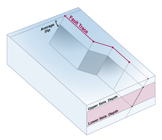
Simple Fault
 (click to enlarge)
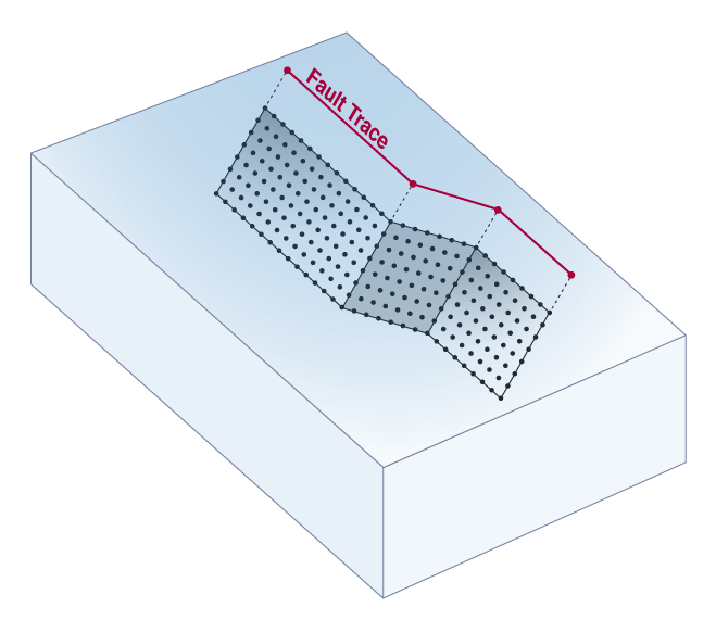
The geometry of a Simple Fault, the most common fault type used in OpenSHA, is described by the fault’s Trace, Average Dip and Upper and Lower Seismogenic Depths. This is the minimum information required to define surfaces on which slip associated with earthquakes occurs. Simple Faults may be gridded according to different algorithms (e.g. see the Frankel and Stirling Fault Surface definitions).
Fault Trace
A line marking the intersection of a fault (rupture) surface with the surface of the earth. In OpenSHA a Fault Trace is represented with a list of locations (latitude, longitude, depth).
Average Dip
The average dip (angle between the earth’s surface and fault plane) along the length of the fault.
Lower Seismogenic Depth
The depth (in km) of the lower limit of seismogenic rupture. This depth is generally based on the maximum depths of microsesmicity in a given region.
Upper Seismogenic Depth
The depth (in km) of the upper limit of seismogenic rupture. This depth is generally applied regionally to reduce near surface seismic energy (moment) release in hazard models (to match observations).
Site
A Site is any location where one is interested in knowing the seismic hazard or risk. Site-specific effects, such as varying shear-wave speed as a function of changing geology, may modulate any computation of hazard.
See also Vs30
Standard Deviation
The type of Standard Deviation used in an Attenuation Relationship calculation. Current options in OpenSHA include:
Total
The total variability.
Inter-Event
The variability from one event to the next.
Intra-Event
The variability among observations within an event.
Zero
Assumes no variability.
Stirling Fault Surface
 (click to enlarge)
A Stirling Fault Surface is one representation of a Gridded Surface as defined by Mark Stirling (and perhaps others). See also Earthquake Rupture. In OpenSHA, the trace and average dip of a Simple Fault are used to create a corrugated surface by translating the Fault Trace down dip, perpendicular to the average fault strike. The resulting surface is then gridded (discretized) according to whatever interval specified is specified. Compare to a Frankel Fault Surface.
Strike, Dip, & Rake (Focal Mechanism)
OpenSHA defines strike, dip and rake according to the conventions set forth by Aki and Richards (1980), Quantitative Seismology, Vol. 1. In OpenSHA, as elsewhere, strike, dip, and rake are used to describe earthquake Focal Mechanisms. Please see the USGS and Wikipedia entries on focal mechanisms for more information.
Strike:
Fault strike is the direction of a line created by the intersection of a fault plane and a horizontal surface, 0° to 360°, relative to North. Strike is always defined such that a fault dips to the right side of the trace when moving along the trace in the strike direction. The hanging-wall block of a fault is therefore always to the right, and the footwall block on the left. This is important because rake (which gives the slip direction) is defined as the movement of the hanging wall relative to the footwall block.
Dip:
Fault dip is the angle between the fault and a horizontal plane, 0° to 90°.
Rake:
Rake is the direction a hanging wall block moves during rupture, as measured on the plane of the fault. It is measured relative to fault strike, ±180°. For an observer standing on a fault and looking in the strike direction, a rake of 0° means the hanging wall, or the right side of a vertical fault, moved away from the observer in the strike direction (left lateral motion). A rake of ±180° means the hanging wall moved toward the observer (right lateral motion). For any rake>0, the hanging wall moved up, indicating thrust or reverse motion on the fault; for any rake<0° the hanging wall moved down, indicating normal motion on the fault.
Examples:
Dip = 90°   Rake = 0°    ::  left-lateral strike-slip
Dip = 90°   Rake = 180°  ::  right lateral strike slip
Dip = 45°   Rake = 90°   ::  reverse fault
Dip = 45°   Rake = -90°  ::  normal fault
See also the Wikipedia and USGS entries on strike and dip.
Tectonic Regime
Earthquakes occur in various tectonic regimes, and models are often tailored to a single regime. Probabilistic earthquake sources state their tectonic regime, which may be used in hazard calculations to select the appropriate GMPEs. Options are:
| Name | OpenSHA Enum Constant |
|---|---|
| Active Shallow Crust | ACTIVE_SHALLOW |
| Stable Shallow Crust | STABLE_SHALLOW |
| Subduction Interface | SUBDUCTION_INTERFACE |
| Subduction IntraSlab | SUBDUCTION_SLAB |
| Volcanic | VOLCANIC |
Wills Site Classification
This is the site-type classification scheme developed by Wills et al. (2000, Bull. Seism. Soc. Am., vol. 90, p. 187-208). The categories and their Vs30 equivalents are:
| Site Class | Vs30 range (m/sec) |
|---|---|
| B | >760 |
| BC | 555-1000 |
| C | 360-760 |
| CD | 270-555 |
| D | 180-360 |
| DE | 90-270 |
| E | <180 |
Copyright ©2026 University of Southern California. All rights reserved. License—Disclaimer
This website is generated automatically from the OpenSHA wiki on GitHub, and is powered by GitHub Pages, Jekyll, and this GitHub Action.